Learning to Solve Parametric Mixed-Integer Optimal Control Problems via Differentiable Predictive Control

1Slovak University of Technology, Slovakia 2Ruhr University Bochum, Germany, 3Johns Hopkins University, USA

Abstract

This paper proposes a novel approach to solving input- and state-constrained parametric mixed-integer optimal control problems using Differentiable Predictive Control (DPC). Our approach follows the differentiable programming paradigm by learning an explicit neural policy that maps control parameters to integer- and continuous-valued decision variables. This policy is optimized via stochastic gradient descent by differentiating the model predictive control objective through the closed-loop finite-horizon response of the system dynamics. To handle integrality constraints, we incorporate three differentiable rounding strategies. The approach is evaluated on a conceptual thermal energy system, comparing its performance with the optimal solution for different lengths of the prediction horizon. The simulation results indicate that our self-supervised learning approach can yield high-quality performance while alleviating training scalability limitations prevalent in imitation learning and significantly reducing inference time by avoiding online optimization.


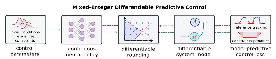
Mixed-Integer Differentiable Predictive Control Diagram

Figure: Conceptual diagram of mixed-integer differentiable predictive control. Green dashed arrows represent the forward pass, while purple dashed arrows represent the backward pass.
Motivation

Mixed-integer optimal control problems (MI-OCPs) arise throughout energy management, robotics, transportation, and industrial process control. In this class of problems, one or more decision variables must take integer or quantized values, so the controller must jointly optimize continuous and discrete inputs while respecting dynamics and constraints.

Constrained MI-OCPs can be solved online as mixed-integer model predictive control (MI-MPC) (McAllister and Rawlings, 2022). With a quadratic stage cost, affine dynamics, and linear constraints, it becomes a mixed-integer quadratic program (MIQP) (Borrelli et al., 2017), whose combinatorial complexity can scale exponentially and is often prohibitive in real time.

In practice this cost is typically reduced at the expense of suboptimality, for example by relaxing optimality along the horizon while keeping integrality (Frick et al., 2015), by dropping integrality along the horizon (Javan et al., 2024), or by warm-starting branch-and-bound (Marcucci and Tedrake, 2021). Learning-based alternatives include imitation of optimal trajectories (Karg and Lucia, 2018; Cauligi et al., 2020), predicting integer decisions and then solving the remaining convex program (Löhr et al., 2020; Reiter et al., 2025; Cauligi et al., 2022), and reinforcement learning over mixed action spaces (Guo et al., 2022; Xu et al., 2025). Multiparametric programming precomputes an explicit solution map (Dua et al., 2002), but scales poorly (Alessio and Bemporad, 2009).

Differentiable Predictive Control (DPC) (Drgoňa et al., 2022, 2024) follows a similar explicit-control idea: a finite-horizon parametric OCP is posed as a differentiable program, and the solution map is a parametric policy trained offline by stochastic gradient descent. This work extends DPC to MI-OCPs by enforcing integrality with differentiable rounding layers, so mixed-integer policies can be trained without online combinatorial search.

Contributions


Problem Formulation

We consider a linear time-invariant discrete-time system \[ x_{k+1} = A x_k + B_u u_k + B_{\delta} \delta_k + E d_k, \] where \( u \in \mathbb{R}^{n_u} \) and \( \delta \in \mathbb{Z}^{n_{\delta}} \) are the continuous- and integer-valued inputs, \( d \in \mathbb{R}^{n_d} \) is a known disturbance, and \( x \in \mathbb{R}^{n_x} \) is the system state. The system is assumed controllable and subject to linear constraints \[ x_k \in \mathcal{X},\quad u_k \in \mathcal{F},\quad \delta_k \in \mathcal{D},\qquad \forall k \ge 0, \] where \( \mathcal{X} \subset \mathbb{R}^{n_x} \) and \( \mathcal{F} \subset \mathbb{R}^{n_u} \) are compact, and \( \mathcal{D} \subset \mathbb{Z}^{n_{\delta}} \) encodes the integrality constraints.

The stage and terminal costs are the weighted squared Euclidean norms of the tracking error and of the continuous and integer inputs, \begin{align} \ell_K(x_k, r_k, u_k, \delta_k) &= \|x_k - r_k\|_Q^2 + \|u_k\|_R^2 + \|\delta_k\|_{\rho}^2, \\ \ell_N(x_k, r_k) &= \|x_k - r_k\|_P^2, \end{align} where \( r \in \mathbb{R}^{n_x} \) is the reference and the weights \( P, Q \) are positive semi-definite while \( R, \rho \) are positive definite.
Mixed-Integer Model Predictive Control
The nominal single-shooting MI-MPC problem is \begin{align} \min_{u,\delta}\quad &\ell_N(x_N, r_N) + \sum_{k=0}^{N-1} \ell_K(x_k, r_k, u_k, \delta_k) \\ \text{s.t.}\quad &x_{k+1} = A x_k + B_u u_k + B_{\delta} \delta_k + E d_k, \\ &u_k \in \mathcal{F},\quad \delta_k \in \mathcal{D}, \qquad \forall k \in \{0,1,\dots,N-1\}, \\ &x_k \in \mathcal{X}, \qquad \forall k \in \{0,1,\dots,N\}, \end{align} where \( N \in \mathbb{Z}_{>0} \) is the prediction horizon. Because of its combinatorial nature, computing the optimal solution may scale exponentially with problem size.
Parametric Mixed-Integer Optimal Control Problem
We recast the problem as a parametric MI-OCP over a policy \( \pi_{\theta} \), \begin{align} \min_{\theta}\quad &\mathbb{E}_{\xi_k \sim P_{\xi}} \Biggl[ \ell_N(x_N, r_N) + \sum_{k=0}^{N-1} \ell_K(x_k, r_k, u_k, \delta_k) \Biggr] \\ \text{s.t.}\quad &x_{k+1} = A x_k + B_u u_k + B_{\delta} \delta_k + E d_k, \\ &\begin{bmatrix} u_k \\ \delta_k \end{bmatrix} = \pi_{\theta}(\xi_k), \\ &u_k \in \mathcal{F},\quad \delta_k \in \mathcal{D}, \qquad \forall k \in \{0,1,\dots,N-1\}, \\ &x_k \in \mathcal{X}, \qquad \forall k \in \{0,1,\dots,N\}. \end{align} The expectation is over control parameters \( \xi_k \) drawn from a known distribution \( P_{\xi} \). For a constant reference, constant constraints, and known future disturbances, this vector is \[ \xi_k = \bigl[ x_k^\top,\; d_k^\top,\; \dots,\; d_{k+N}^\top \bigr]^\top \in \mathbb{R}^{n_{\xi}}. \] The policy \( \pi_{\theta}: \mathbb{R}^{n_{\xi}} \to \mathbb{R}^{n_u} \times \mathbb{R}^{n_{\delta}} \) maps \( \xi_k \) to mixed-integer inputs, and the dynamics generate an \( N \)-step closed-loop rollout used to evaluate the MPC objective.

Methodology

DPC formulates the parametric OCP as a differentiable program (Drgoňa et al., 2022, 2024). State and input constraints are relaxed with a penalty method, yielding \begin{align} \min_{\theta}\quad &\mathbb{E}_{\xi_k \sim P_{\xi}} \Biggl[ \|x_N - r_N\|_P^2 + \sum_{k=0}^{N-1} \Bigl( \|x_k - r_k\|_Q^2 + \|u_k\|_R^2 + \|\delta_k\|_{\rho}^2 + c_x\, q(x_k, x_N) + c_u\, p(u_k, \delta_k) \Bigr) \Biggr] \\ \text{s.t.}\quad &x_{k+1} = A x_k + B_u u_k + B_{\delta} \delta_k + E d_k, \\ &\begin{bmatrix} u_k \\ \delta_k \end{bmatrix} = \pi_{\theta}(\xi_k), \end{align} where \( q(\cdot) \) and \( p(\cdot) \) are constraint-violation norms with weights \( c_x \) and \( c_u \).

If the dynamics and policy are differentiable, \( \theta \) can be optimized with stochastic gradient descent. Gradients of the total loss \( \ell \) follow from the chain rule, \begin{align} \nabla_{\theta} \ell &= \frac{\partial \ell_K}{\partial \theta} + \frac{\partial \ell_N}{\partial \theta} + \frac{\partial q(x)}{\partial \theta} + \frac{\partial p(u,\delta)}{\partial \theta} \\ &= \frac{\partial \ell_K}{\partial x}\frac{\partial x}{\partial u}\frac{\partial u}{\partial \theta} + \frac{\partial \ell_K}{\partial x}\frac{\partial x}{\partial \delta}\frac{\partial \delta}{\partial \theta} + \frac{\partial \ell_K}{\partial u}\frac{\partial u}{\partial \theta} + \frac{\partial \ell_K}{\partial \delta}\frac{\partial \delta}{\partial \theta} \\ &\quad + \frac{\partial \ell_N}{\partial x}\frac{\partial x}{\partial u}\frac{\partial u}{\partial \theta} + \frac{\partial \ell_N}{\partial x}\frac{\partial x}{\partial \delta}\frac{\partial \delta}{\partial \theta} + \frac{\partial q(x)}{\partial x}\frac{\partial x}{\partial u}\frac{\partial u}{\partial \theta} \\ &\quad + \frac{\partial q(x)}{\partial x}\frac{\partial x}{\partial \delta}\frac{\partial \delta}{\partial \theta} + \frac{\partial p(u)}{\partial u}\frac{\partial u}{\partial \theta} + \frac{\partial p(\delta)}{\partial \delta}\frac{\partial \delta}{\partial \theta}, \end{align} where \( \partial u / \partial \theta \) and \( \partial \delta / \partial \theta \) are obtained by backpropagation through time (Puskorius and Feldkamp, 1994). The remaining obstacle is that a mixed-integer policy is not differentiable. We therefore insert a discrete output layer and approximate its Jacobian with a Straight-Through Estimator (STE) (Bengio et al., 2013): the forward pass uses a non-differentiable rounding map, while the backward pass uses a smooth surrogate.

The policy is a feed-forward network with a shared latent encoder and two heads, \begin{align} h_k &= f^{(h)}_{\theta^{(h)}}(\xi_k), \\ y^{(u)}_k &= f^{(u)}_{\theta^{(u)}}(h_k), \\ y^{(\delta)}_k &= f^{(\delta)}_{\theta^{(\delta)}}(h_k), \end{align} where \( f^{(h)}_{\theta^{(h)}}: \mathbb{R}^{n_{\xi}} \to \mathbb{R}^{n_h} \) lifts the control parameters and the heads produce relaxed continuous and integer decisions. The trainable parameters are \( \theta = \{\theta^{(h)}, \theta^{(u)}, \theta^{(\delta)}\} \).
Straight-Through Estimator with Sigmoid
Integrality is enforced by rounding the relaxed integer output to the nearest integer, \begin{align} \delta_k &= \bigl\lfloor y^{(\delta)}_k \bigr\rceil, \\ u_k &= y^{(u)}_k. \end{align} The backward pass uses a slope-parameterized sigmoid \( \sigma(x) = \bigl(1 + e^{-\eta x}\bigr)^{-1} \) with \( \eta \in \mathbb{R}_{\ge 1} \). Larger \( \eta \) matches the rounding discontinuity more closely, at the cost of steeper gradients. The STE approximation is \begin{align} \nabla \delta_k &\approx \nabla \sigma\bigl(\eta\bigl(y^{(\delta)}_k - \lfloor y^{(\delta)}_k \rfloor - t\bigr)\bigr) \\ &\approx \sigma\bigl(\eta\bigl(y^{(\delta)}_k - \lfloor y^{(\delta)}_k \rfloor - t\bigr)\bigr) \Bigl( 1 - \sigma\bigl(\eta\bigl(y^{(\delta)}_k - \lfloor y^{(\delta)}_k \rfloor - t\bigr)\bigr) \Bigr) \eta, \end{align} with rounding threshold \( t = 0.5 \). This construction applies when feasible integers are evenly spaced, e.g. \( \{0,1,2\} \). Uneven sets such as \( \{0,1,5\} \) are better handled categorically.
Straight-Through Estimator with Softmax
The integer decision is treated as a categorical classification. The relaxed output is a collection of score vectors, one per integer input, \[ y^{(\delta)}_k = \{ S_{k|j} \}_{j=1}^{n_{\delta}}, \qquad S_{k|j} = [s_{k|1},\dots,s_{k|L_j}]^\top, \qquad L_j \ge 2, \] where \( s_{k|i} \) is the score of feasible integer index \( i \in \{1,\dots,L_j\} \). Scores are turned into probabilities with a Gumbel-Softmax (Jang et al., 2017), \begin{align} \hat{s}_{k|i} &= \frac{ \exp\bigl((\log s_{k|i} + g_{k|i})\,\tau^{-1}\bigr) }{ \sum_{m=1}^{L_j} \exp\bigl((\log s_{k|m} + g_{k|m})\,\tau^{-1}\bigr) }, \qquad \forall i \in \{1,\dots,L_j\}, \\ \hat{S}_{k|j} &= [\hat{s}_{k|1},\dots,\hat{s}_{k|L_j}]^\top, \qquad \hat{s}_{k|i} \in (0,1), \end{align} where \( g_{k|i} \sim \mathrm{Gumbel}(0,1) \) and \( \tau \in \mathbb{R}_{>0} \) is a temperature. If \( \tau < 1 \), the probability vector polarizes, and \( \sum_m \hat{s}_{k|m} = 1 \).

Let \( \mathcal{A} = \{ A_j \}_{j=1}^{n_{\delta}} \) collect admissible integer vectors \( A_j = [a_1,\dots,a_{L_j}]^\top \). A one-hot encoding of the Gumbel-Softmax sample selects exactly one admissible value, \begin{align} \bar{s}_{k|i} &= \begin{cases} 1, & \text{if } i = \arg\max_m \hat{s}_{k|m}, \\ 0, & \text{otherwise,} \end{cases} \\ \delta_k &= \bigl[ \bar{S}_{k|1}^\top A_1,\; \dots,\; \bar{S}_{k|n_{\delta}}^\top A_{n_{\delta}} \bigr]^\top. \end{align} Because one-hot encoding is non-differentiable, the backward pass replaces \( \bar{S} \) by the polarized probabilities, \[ \nabla \delta_k \approx \Bigl[ \nabla\bigl(\hat{S}_{k|1}^\top A_1\bigr),\; \dots,\; \nabla\bigl(\hat{S}_{k|n_{\delta}}^\top A_{n_{\delta}}\bigr) \Bigr]^\top. \] As \( \tau \to 0 \) the surrogate matches the discrete map more closely, at the expense of numerical stability.
Learnable Threshold Approach
The learnable-threshold (LT) method of Tang et al. (2025) predicts a continuous relaxation with one network, \( y^{(\delta)}_k = \phi_{1|\theta_1}(\xi_k) \), and a correction with a second network, \( q_k = \phi_{2|\theta_2}(\xi_k, y^{(\delta)}_k) \), so that \( y^{(\delta)}_k \leftarrow y^{(\delta)}_k + q_k \). Rounding thresholds are obtained from predicted logits as \( t_k = \sigma(z_k) \). The integer input is then \[ \delta_k = \begin{cases} \lfloor y^{(\delta)}_k \rfloor, & \text{if } y^{(\delta)}_k - \lfloor y^{(\delta)}_k \rfloor < t_k, \\[4pt] \lceil y^{(\delta)}_k \rceil, & \text{otherwise.} \end{cases} \] Gradients of this rounding map are again approximated with a sigmoid STE, now with a learnable threshold in place of the fixed value \( t = 0.5 \).

Numerical Example

The method is demonstrated on a second-order linear thermal system with two continuous inputs, one integer input, and two known disturbances, inspired by Löhr et al. (2019). The system matrices are \[ A = \begin{bmatrix} \alpha_1 & \nu \\ 0 & \alpha_2 - \nu \end{bmatrix},\quad B_u = \begin{bmatrix} b_1 & 0 \\ 0 & b_2 \end{bmatrix},\quad B_{\delta} = \begin{bmatrix} 0 \\ b_3 \end{bmatrix},\quad E = \begin{bmatrix} -b_4 & 0 \\ 0 & -b_5 \end{bmatrix}. \] Here \( \alpha_1 = 0.9983 \) and \( \alpha_2 = 0.9966 \) are dissipation rates of thermal storage tanks \( x_1 \) and \( x_2 \), \( \nu = 0.001 \) is the energy-transfer rate from tank \( x_2 \) to tank \( x_1 \), and \( b_1 = b_2 = 0.075 \) are heat-pump efficiencies for \( u_1 \) and \( u_2 \). The integer input \( \delta_1 \in \{0,1,2,3\} \) is the number of active \( 1\,\mathrm{kW} \) heating rods in tank \( x_2 \), with efficiency \( b_3 = 0.0825 \). Disturbance gains are \( b_4 = b_5 = 0.0833 \). These parameters correspond to a sampling period \( T = 300\,\mathrm{s} \).

Tracking is weighted by \( Q = \mathrm{diag}(1,1) \) for both stage and terminal costs (\( P = Q \)). Continuous inputs are penalized by \( R = \mathrm{diag}(0.5, 0.5) \) and the integer input by \( \rho = 0.1 \). These weights are chosen for a clear benchmark rather than a real-world cost: heating rods are cheaper than the heat pumps so that integer actuation is used frequently. States are constrained to \( 0 \le x_1 \le 8.4 \) and \( 0 \le x_2 \le 3.6 \) with penalty \( c_x = 25 \). Continuous inputs satisfy \( u_1, u_2 \ge 0 \) and \( 0 \le u_1 + u_2 \le 8 \) with penalty \( c_u = 25 \). The references are the constant setpoints \( r_1 = 4.2 \) and \( r_2 = 1.8 \).
Controller Synthesis
Training uses a synthetic dataset of control parameters \( \xi \), containing initial states and an \( N \)-step window of future disturbances. Initial conditions are sampled uniformly over the state bounds, \( x_{1|0} \sim \mathcal{U}(0, 8.4) \) and \( x_{2|0} \sim \mathcal{U}(0, 3.6) \). Disturbance \( d_1 \) is drawn from a scaled Beta law, \( d_{1|0,\dots,N} \sim \mathrm{Beta}(0.6, 1.4) \) multiplied by \( 7 \), matching the test data. Disturbance \( d_2 \) is a peak signal with amplitudes in \( [1, 16] \) and durations of \( 2 \) to \( 5 \) steps.

All policies are trained on \( 24{,}000 \) samples with \( 4{,}000 \) held out for validation, using batch size \( n_b = 2000 \) and Adam with learning rate \( \zeta = 3 \times 10^{-4} \). Each training step performs a single-shooting closed-loop rollout: the policy is evaluated, integer outputs are rounded, the linear dynamics are stepped, and the disturbance window is shifted with zero padding. Gradients of the MPC loss are then backpropagated through the rollout and used to update \( \theta \). Policies and simulations were obtained with NeuroMANCER v1.5.6 and PyTorch v2.8.0.
Simulation Results
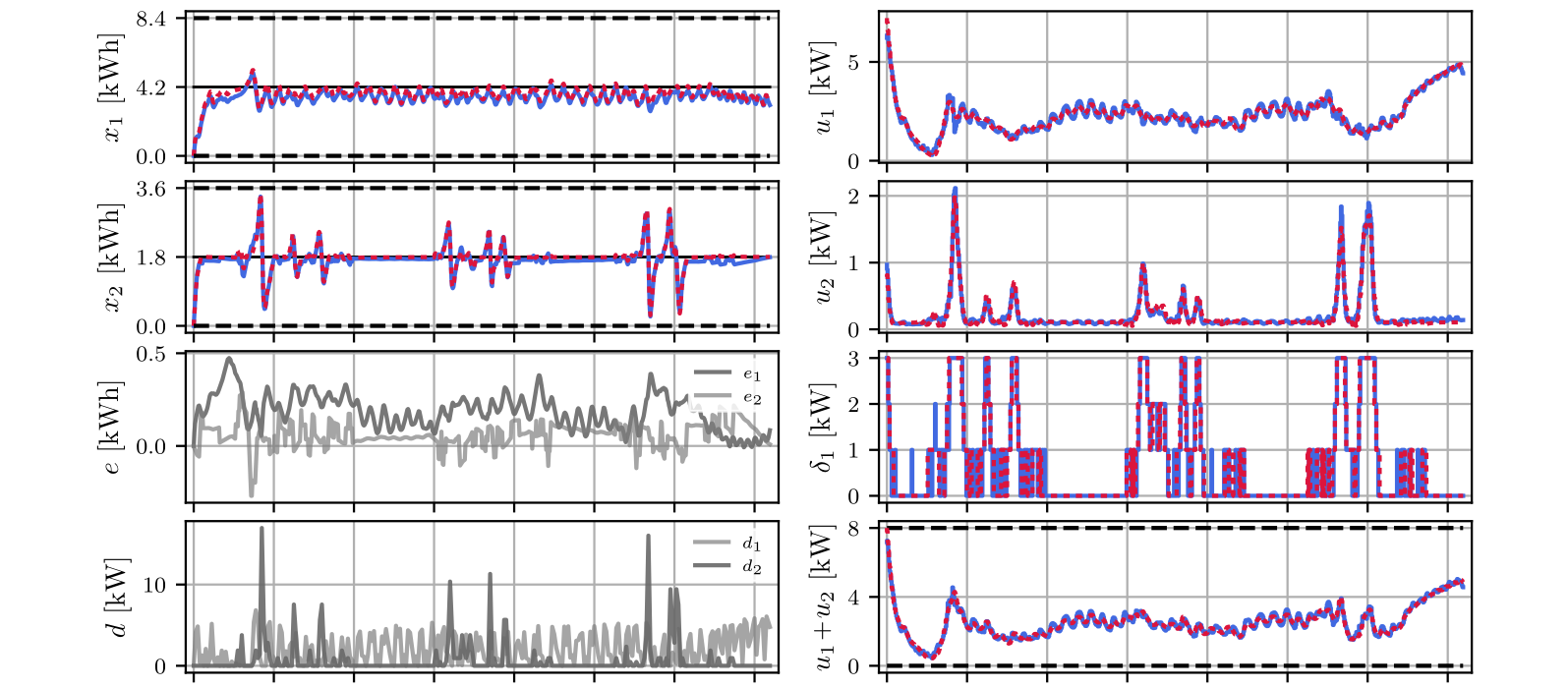
Closed-loop receding-horizon simulations of \( 1872 \) steps (\( 6.5 \) days) were run from \( 20 \) initial conditions. The figure below compares MI-DPC with Sigmoid STE to the optimal MIQP trajectories for \( N = 20 \). The quantities \( e_1 \) and \( e_2 \) are the differences between the optimal and MI-DPC state trajectories.

Closed-loop simulation results of MI-DPC versus the optimal MIQP solution

Figure: Closed-loop simulation results obtained with MI-DPC with Sigmoid STE (blue), compared with the optimal solution (dashed red), for \( N = 20 \). Reference states are depicted in black and state/input bounds in dashed black.


Performance is summarized by the mean closed-loop stage cost \[ \ell_{\mathrm{mean}} = (n_{\mathrm{ic}} n_{\mathrm{sim}})^{-1} \sum_{i=1}^{n_{\mathrm{ic}}} \sum_{k=0}^{n_{\mathrm{sim}}} \ell_K(x_{k|i}, u_{k|i}, \delta_{k|i}), \] where \( n_{\mathrm{ic}} \) is the number of initial conditions and \( n_{\mathrm{sim}} \) is the simulation length. Relative suboptimality margin (RSM) is reported against the hard-constrained MIQP solved with CPLEX v22.1.2.
Table: Comparison of methods for solving the MI-OCP with varying prediction horizon \( N \).
Approach Metric \(10\) \(15\) \(20\) \(25\) \(30\) \(40\)
MI-DPC with Sigmoid STE \(\ell_{\mathrm{mean}}\) 6.824.604.193.953.893.85
RSM (%) 14.314.144.371.421.15–
MIT (s)1 0.00020.00020.00020.00020.00020.0002
NTP 826038400385403868038820391003
TT (s)2 231.6347.5214.4440.8410.3444.1
MI-DPC with Softmax STE \(\ell_{\mathrm{mean}}\) 6.764.794.113.933.903.86
RSM (%) 13.568.052.361.111.36–
MIT (s)1 0.00020.00020.00020.00020.00020.0002
NTP 830268442685826872268862691426
TT (s)2 223.3281.6373.3432.7317.3393.36
MI-DPC with Learnable Threshold \(\ell_{\mathrm{mean}}\) 6.424.534.083.903.863.84
RSM (%) 8.962.691.680.450.41–
MIT (s)1 0.00040.00040.00040.00040.00040.0004
NTP 781918009181991838918579189591
TT (s)2 429.9573.8664.6845.7821.41080.9
Imitation learning with Sigmoid STE \(\ell_{\mathrm{mean}}\) 5.874.484.063.963.894.99
RSM (%) 0.521.521.151.921.27–
MIT (s)1 0.00020.00020.00020.00020.00020.0002
NTP 826038400385403868038820391003
TT (s)3 1826.92335.23645.94405.67053.27238.9
Optimal (MIQP4) \(\ell_{\mathrm{mean}}\) 5.844.414.013.883.84\(\dagger\)
MIT (s)1 0.00310.00850.04210.25071.3140\(\dagger\)
FUP (%) 0000.042.44\(\dagger\)

Acronyms: RSM – relative suboptimality margin; MIT – mean inference time; NTP – number of trainable parameters; TT – training time; FUP – fraction of unsolved problems within a \( 15\,\mathrm{s} \) limit.
1 Measured using a single thread of Intel Core i9-14900KF. 2 Trained using an NVIDIA GeForce RTX 5090. 3 Includes time to compute the labeled training set (2-hour limit) and neural policy training. 4 Solved with the CPLEX branch-and-bound algorithm. \( \dagger \) Failed to complete simulations within 20 hours; based on 100 samples, MIT is estimated at \( 14.3\,\mathrm{s} \).



The RSM of MI-DPC decreases as the horizon grows: longer rollouts let backpropagation see more of the transient dynamics, so the explicit policy better approximates the parametric MI-OCP. Inference time stays essentially constant because the network architecture is unchanged across \( N \). Throughout these simulations MI-DPC produced no state- or input-constraint violations, although feasibility is not guaranteed. CPLEX, by contrast, exceeded a \( 15\,\mathrm{s} \) per-step time budget on a fraction of problems for longer horizons.

For \( N = 30 \), MI-DPC reduces mean inference time by four orders of magnitude relative to CPLEX while operating at about \( 1\% \) RSM. The \( N = 40 \) MIQP comparison is omitted because CPLEX was prohibitively slow. Imitation learning with the same Sigmoid STE architecture can outperform DPC at short horizons, but only after a costly labeling phase. At \( N = 40 \) it fails because too few labeled samples can be generated within a two-hour budget. This is the main practical advantage of self-supervised DPC: it avoids solving MIQPs to build a training set.

Conclusions and Future Work

This work introduces a scalable approach to parametric mixed-integer optimal control by embedding differentiable rounding layers in DPC. Integrality is enforced by non-differentiable operations such as rounding, while STE surrogates make the policy trainable by gradient descent. Closed-loop experiments show near-optimal performance with inference several orders of magnitude faster than online MIQP, which makes embedded and edge implementations plausible.

The method does not guarantee closed-loop stability, global optimality, or feasibility, so process-safety applications should pair it with a certified backup controller or safety filter. Future work will target stability and feasibility certificates, and will study larger systems with nonlinear dynamics and constraints.

Acknowledgment

This work was supported by the European Union's Horizon Europe programme under grant no. 101079342 and by the Ralph O’Connor Sustainable Energy Institute (ROSEI) at Johns Hopkins University. J.B. and M.G. also acknowledge the Scientific Grant Agency of the Slovak Republic under grant 1/0401/26, and the Slovak Research and Development Agency under project APVV-22-0436.
FrontSeat, Horizon Europe grant no. 101079342
Slovak University of Technology in Bratislava
Ruhr University Bochum Chair of Automatic Control and Systems Theory, Ruhr University Bochum
Ralph O'Connor Sustainable Energy Institute, Johns Hopkins University

BibTeX

@article{boldocky2025learning,
  title={Learning to Solve Parametric Mixed-Integer Optimal Control Problems via Differentiable Predictive Control},
  author={Boldock{\'y}, J{\'a}n and Javan, Shahriar Dadras and Gulan, Martin and M{\"o}nnigmann, Martin and Drgo{\v{n}}a, J{\'a}n},
  journal={arXiv preprint arXiv:2506.19646},
  year={2025}
}