Data Center Chiller Plant Optimization via Mixed-Integer Nonlinear Differentiable Predictive Control

1Pacific Northwest National Laboratory, 2Slovak University of Technology, 3Johns Hopkins University

Abstract

This paper presents a computationally tractable framework for real-time predictive control of multi-chiller plants whose operation involves discrete and continuous control decisions coupled through nonlinear dynamics, resulting in a mixed-integer optimal control problem. To address this challenge, the Differentiable Predictive Control (DPC)-a self-supervised, model-based learning methodology for approximately solving parametric optimal control problems—is extended to accommodate mixed-integer control policies. The proposed framework is benchmarked against a state-of-the-art mixed-integer Model Predictive Control (MPC) solver and a fast heuristic Rule-Based Controller (RBC). Simulation results demonstrate that the proposed approach achieves significant energy savings over the RBC while maintaining orders-of-magnitude faster computation times than MPC, offering a scalable and practical alternative to conventional combinatorial mixed-integer control formulations.


Neural DAE architecture

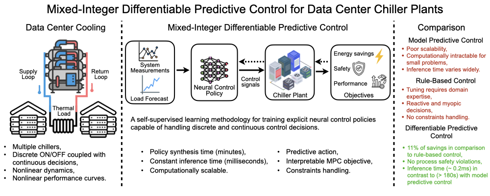
Figure: Graphical Abstract.

Motivation

The rapid expansion of artificial intelligence and digital infrastructure has led to a sharp increase in global data center electricity demand. In the United States alone, data centers currently consume about 150 TWh of electricity annually and are projected to grow to between 200 TWh and 500 TWh by 2030 (Aljbour et al., 2024). With this expansion comes an accompanying demand for high-efficiency cooling systems in data centers. Chiller plants are commonly deployed to perform this task. A chiller plant typically includes heat pumps, pumps, and cooling towers, with the heat pumps being the most energy-intensive components within the plant. Control of chiller plants involves both continuous decision variables (e.g., chilled water supply temperature, differential pressure) and discrete decision variables (e.g., number of chillers active, pump mode). Optimizing these coupled decisions can significantly reduce electricity consumption, ensure reliable operation, and extend the lifespan of costly mechanical assets. However, this requires solving a high-dimensional mixed-integer nonlinear optimal control problem, which is computationally challenging to solve in real time.

To address these challenges, the proposed approach utilizes Differentiable Predictive Control (DPC) (Drgona et al., 2022), which formulates parametric MPC problems as differentiable programs, enabling offline self-supervised learning of explicit neural control policies through gradient-based learning. Expanding upon this foundation, recent work on Mixed-Integer DPC (MI-DPC) (Boldocky et al., 2025) extended this idea to handle mixed-integer optimal control problems (MI-OCPs) with discrete decision variables.

Contributions

  • Formulation of a control-oriented multi-chiller dynamics model.
  • Implementation of mixed-integer differentiable predictive control (MI-DPC) for multi-chiller plant optimization.
  • Introduction of binary-variance regularization (BVR) to limit high frequency binary switching.
  • Performance comparison with rule-based control (RBC) and mixed-integer model predictive control (MI-MPC).
  • Release of open-source code for reproducible numerical experiments.


Problem Formulation

The continuous-time thermal dynamics of the multi-chiller system are \begin{align} Q^{(i)}(t) &= \eta_\mathrm{r}\dot{m}^{(i)}(t)\; c_\mathrm{p}\delta^{(i)}(t) \left( T_\mathrm{r}(t)-T^{(i)}_\mathrm{s}(t) \right), \label{eq:cooling_delivered}\\ \dot{T}_\mathrm{r}(t) &= \frac{1}{C_\mathrm{r}}\left(\tilde{Q}_\text{load}(t) - \sum_{i=1}^{M}Q^{(i)}(t) \right), \label{eq:temp_return}\\ \dot{T}_\mathrm{s}^{(i)}(t) &= -\frac{c_\mathrm{p} \eta_\mathrm{s}}{C^{(i)}}\left(\delta^{(i)}(t)\dot{m}^{(i)}(t) \left(T^{(i)}_\mathrm{s}(t)-T^{(i)}_\mathrm{e}(t)\right)\right),\!\! \label{eq:temp_supply} \end{align}
where \( Q^{(i)}(t)\!\in\!\mathbb{R}_{\ge0} \) is the delivered cooling from chiller \( i \) at time \( t \), \( \delta^{(i)}(t)\!\in\!\{0,1\} \) denotes the chiller's on/off state, \( c_\mathrm{p}\! \in\!\mathbb{R}_{>0} \) is the specific heat capacity of the coolant, \( T_\mathrm{r}(t)\!\in\!\mathbb{R} \) is the return water temperature, and \( C_\mathrm{r},C^{(i)}\!\in\!\mathbb{R}_{>0} \) are the thermal capacitances of the return and chiller loops, \( T_\mathrm{s}^{(i)}(t)\!\in\!\mathbb{R} \) is the supply water temperature for chiller \( i \in \{1, ..., M\} \). Moreover, \( \eta_\mathrm{r},\eta_\mathrm{s}\!\in\!(0,1) \) denote the heat-exchanger efficiency coefficients, and \( \tilde{Q}_\text{load}(t)\!\in\! \mathbb{R}_{\ge0} \) is the effective thermal load, estimated using a low-pass, discrete-time finite impulse response (FIR) filter \( \tilde{Q}_\text{load} (t) = \sum_{l=0}^{L} h_l Q_\text{load}(t-l\Delta t) \), where \( Q_\text{load}(t)\in\mathbb{R}_{\ge 0} \) is the direct server load; an exogenous variable in this context. In the following, the continuous-time dynamics are discretized using a fourth-order Runge-Kutta method with a time-step length \( \Delta t \) and discrete time index \( k \); denoted as \( f(x_k, u_k, \tilde{Q}_{\text{load},k}, \Delta t) : \mathbb{R}^{n_x} \times \mathbb{R}^{n_u} \times \mathbb{R} \rightarrow \mathbb{R}^{n_x} \), where \( x_k = [T_r(k), T_s^{(1)}(k), ..., T_s^{(M)}(k)]^T \).

The power consumption of chillers \( P^{(i)}_\text{chiller}(t)\in\mathbb{R}_{\ge 0} \) and pumps \( P^{(i)}_\text{pump}(t)\in\mathbb{R}_{\ge 0} \) are modeled as \begin{align} P^{(i)}_\text{chiller}(t) &= \frac{Q^{(i)}(t)}{\text{COP}^{(i)}(t)}+\rho^{(i)}\delta^{(i)}(t) \label{eq:chiller_power},\\ \text{COP}^{(i)}(t) &= a_0^{(i)}+a_1^{(i)}\frac{Q^{(i)}(t)}{Q_\text{max}^{(i)}}+a_2^{(i)}\left(\frac{Q^{(i)}(t)}{Q_\text{max}^{(i)}}\right)^2,\\ P^{(i)}_\text{pump}(t) &= \gamma^{(i)}\left( \dot{m}^{(i)}(t)\delta^{(i)}(t) \right)^3, \label{eq:pump_power} \end{align} for the system constants \( a_{0:2}^{(i)},\gamma^{(i)},\rho^{(i)},Q_\text{max}^{(i)}\!\in\!\mathbb{R} \). The constant \( \rho \) represents the base power required for chiller operation. In this formulation, the chiller's coefficient of performance \( \text{COP}^{(i)}(t)\in\mathbb{R}_{\ge0} \) is a function of the part-load ratio (PLR), the ratio of current cooling to maximum cooling capacity. Ensuring that each chiller is operating near its highest efficiency load ratio is the core of the underlying optimal control problem.
Schematic diagram of the multi-chiller system

Figure: Schematic of a multiple-chiller plant arranged in a parallel configuration.

Methodology

We formulate the mixed-integer optimal control problem as a differentiable program:
\begin{align} \nonumber \min_{\theta_1,\theta_2,\theta_3}\mathbb{E}_{ \xi \sim P_{ \xi} }\! &\bigg[\sum_{k=0}^{N-1} \sum^M_{i=1} \underbrace{P^{(i)}_{\text{chiller},k}}_{\text{chiller power}}\!+\! \underbrace{P^{(i)}_{\text{pump},k}}_{\text{pump power}}\!+\! \underbrace{\|\Delta\delta_k\|_R^2}_{\substack{\text{switching} \\ \text{penalty}}} \!+\! \lambda_W \underbrace{\left(Q_k\!-\!Q_{\text{load},k}\right)^2}_{\text{load tracking}} \!+\! \underbrace{\lambda_x q(x_k)}_{\substack{\text{state cosntr.} \\ \text{penalty}}} \!+\! \underbrace{\lambda_u p(u_k)}_{\substack{\text{input constr.} \\ \text{penalty}}} \!+\! \underbrace{\|\tilde\delta_k\odot(1-\tilde\delta_k)\|^2_\Lambda}_{\substack{\text{binary-variance} \\ \text{regularization}}}\bigg]\\[-0pt] {\text{subject to}} \nonumber\\[-0pt] \; x_{k+1}=&f\left(x_k, u_k,\tilde{Q}_{\text{load},k}, \Delta t\right), \label{eq:dpc-dynamics} \textcolor{gray}{\leftarrow\text{dynamics}}\\ \dot{m}_k\!=&\,\pi_{\theta_1}(\xi_k),\; \textcolor{gray}{\leftarrow\text{mass flow rate decision}}\\ T_{\mathrm{e},k}\!=&\,\pi_{\theta_2}(\xi_k),\; \textcolor{gray}{\leftarrow\text{evaporation temperature decision}}\\ \tilde\delta_k\!=&\,\pi_{\theta_3}(\xi_k), \textcolor{gray}{\leftarrow\text{relaxed binary decision}}\\ \delta_k \in &\;\{0,1\}^M, \;\, \forall k \in \{0,\dots,N\!-\!1\},\label{eq:dpc-binary} \textcolor{gray}{\leftarrow\text{integrality constraint}}\\ \delta^{(2)}_k =& \,1,\;\quad\quad\quad \forall k\in\{0,\dots,N-1\}, \label{eq:dpc-oneon} \textcolor{gray}{\leftarrow\text{"one-ON" safety constraint}}\\ \xi_k\!:=&\!\;[x_k, \tilde{Q}_{\text{load},k}, Q_{\text{load},k},\dots,Q_{\text{load},k\!+\!N}]^\top\!\!\!. \textcolor{gray}{\leftarrow\text{control parameters vector}}\label{eq:dpc-xi}\end{align}

where, the parameters \( \theta_{(\cdot)} \) of the control policies \( \pi_{\theta_1} \), \( \pi_{\theta_2} \), and \( \pi_{\theta_3} \) are the optimization arguments. The policies map the vector of control parameters \( \xi \) to continuous-valued control variables \( \dot m \) (mass flow), \( T_\mathrm{e} \) (evaporation temperature), and a slack variable \( \tilde\delta\!\in\!\mathbb{R}^{M-1} \) (relaxed value of the binary control variable \( \delta \)). By fixing one of the binary variables, the dimension of \( \tilde\delta \) is reduced to \( M\!-\!1 \). This is done as a safety mechanism to ensure that at least one chiller is always on. To compute control variables, separate neural modules are used, which are represented by fully connected deep neural networks. Moreover, the control parameters are sampled from a known probability distribution \( P_\xi \) to emulate scenarios that are likely to occur during the system's operation. \(N\) denotes prediction horizon length, whereas functions \( q(\cdot) \) and \( p(\cdot) \) denote state and input penalty functions weighted by \( \lambda_x \) and \( \lambda_u \), respectively.

The binary integrality is enforced using a threshold-based discretization scheme with a fixed threshold of \(0.5\), given as \begin{align} \delta^{(i)}_{k} = & \begin{cases} 1, & \text{if } \tilde\delta^{(i)}_{k}>0.5,\\[0pt] 0, & \text{otherwise.}\\[0pt] \end{cases} \end{align} This function behaves analogously to a Heaviside function exhibiting a discontinuity at \(0.5\). To enable gradient-based optimization, a Straight-through estimator heuristic by (Bengio et al., 2013), is used. The gradient is approximated using its differentiable surrogate, given by a scaled sigmoid function \( \sigma(x)\!=\!\left(1+e^{-\mu (x-0.5)} \right)^{-1} \), where \( \mu\!\in\!\mathbb{R}_{>0} \) is a slope parameter determining the sharpness of the transition; additionally, the function is centered at \(0.5\). Accordingly, the derivative is approximated as \begin{align} \frac{\partial \delta^{(i)}_{k}}{\partial \tilde{\delta}^{(i)}_{k}} \approx \frac{\partial \sigma\!\left(\tilde{\delta}^{(i)}_{k}\right)}{\partial \tilde{\delta}^{(i)}_{k}}. \end{align}
The differentiable computational graph, comprises four components: a continuous neural policy, a differentiable rounding layer, a differentiable ordinary differential equation (ODE) solver, and a model predictive loss function. Given synthetically sampled control parameters that include the initial conditions and a length-\(N\) vector of exogenous variables (server load), a closed-loop rollout of length \(N\) is performed through the integrated system dynamics, constituting the single-shooting forward pass. Consequently, the loss function is evaluated based on the resulting closed-loop trajectories. The backward pass is used to enable policy optimization by propagating gradients through the computational graph. Specifically, gradients of the loss function with respect to policy parameters are obtained by back-propagating through the integrated system dynamics using either the backpropagation through time algorithm (Puskorius and Feldkamp, 1994).
MI-DPC Architecture

Figure: Conceptual diagram of the mixed-integer differentiable predictive control for nonlinear chiller plant optimization. Green dashed arrows represent the forward pass, while red dashed arrows represent the backward pass.
Binary-Variance Regularization
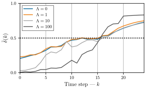
To promote binary polarization of the relaxed variable \( \tilde \delta \) and to complement the \( \Delta\delta \) penalty in suppressing high-frequency switching, a binary-variance regularization (BVR) is introduced as \( \|\tilde\delta_k\odot(1-\tilde\delta_k)\|_\Lambda^2 \), where \( \Lambda\!\in\!\mathbb{R}^{M-1\times M-1} \) denotes the weighting matrix. As the weight increases, the regularization penalizes values of \( \tilde\delta \) near the discretization threshold (\(0.5\)), as well as those outside the \([0,1]\) range. Based on extensive numerical experiments, this regularization has proven crucial to the proposed framework, as its omission leads to \( \tilde\delta \) values clustering around the discretization threshold, thereby increasing the likelihood of high-frequency switching behavior. The influence of this regularization on the relaxed binary variable for different penalty magnitudes is illustrated in the following Figure.
BVR

Figure: Experimental results for the influence of the binary-variance regularization on the relaxed binary variable for different penalty magnitudes under a step change in cooling load from \(150 \text{ kW}\) to \(500 \text{ kW}\) occurring at time \( k\!=\!20 \).

Simulation Results

Our chiller plant optimization framework and all our examples are implemented using the Neuromancer library.

Let's consider optimization problem of multi-chiller plant with sampling time of \( \Delta t = 180 \) seconds and the following parameters:

Table: Chiller system parameters.
Symbol Description Value Unit
\(c_\mathrm{p}\) Specific heat of water 4.184 kJ/(kg·°C)
\(C\) Thermal capacitance 14644 kJ/°C
\(C_\mathrm{r}\) Thermal capacitance 29288 kJ/°C
\(\rho\) Base chiller power 10 kW
\(Q_{\max}\) Maximum rated cooling 500 kW
\(a_0\) Efficiency coefficient 1 -
\(a_1\) Efficiency coefficient 19.33 -
\(a_2\) Efficiency coefficient -18.33 -
\(\eta_\mathrm{s}\) Heat exchanger efficiency 0.7 -
\(\eta_\mathrm{r}\) Heat exchanger efficiency 0.75 -
\(\gamma\) Pump power coefficient 9.62e-4 kW·s³/kg³
\(\dot{m}^\text{min}\) Minimum mass flow rate 6 kg/s
\(\dot{m}^\text{max}\) Maximum mass flow rate 20 kg/s
\(T_\text{s}^{\text{min}}, T_\text{e}^{\text{min}}, T_\text{r}^{\text{min}}\) Minimum temperatures 7 °C
\(T_\text{s}^{\text{max}}, T_\text{e}^{\text{max}}\) Maximum temperatures 12 °C
\(T_\text{r}^{\text{max}}\) Maximal return temp. 26 °C
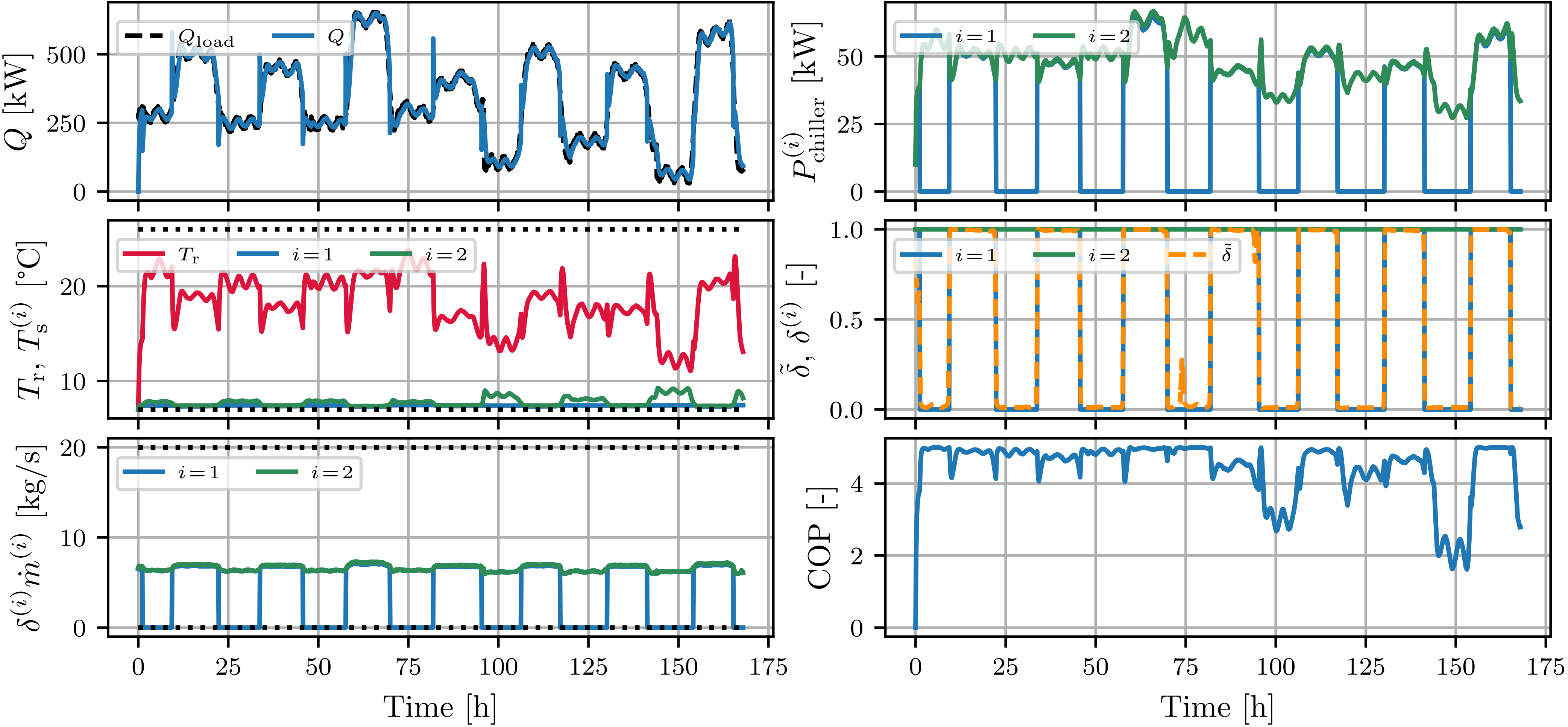
The closed-loop response of the MI-DPC controller, implemented in a receding-horizon manner, is shown in the Figure below. The results illustrate that the controller tracks the time-varying cooling demand over the seven-day simulation while coordinating the chiller power consumption, return and supply temperatures, binary staging decisions, and mass flow rates. Around \(75\) hours, the relaxed integer variable \(\tilde{\delta}\) increases toward the rounding threshold, indicating that the controller temporarily favors activating the second controllable chiller. This behavior is consistent with the PLR-COP characteristic: operating an additional unit may improve chiller efficiency by shifting the active chillers toward a more favorable part-load ratio. However, \(\tilde{\delta}\) remains below the rounding threshold, so the additional chiller is not activated. This suggests that, within the predictive objective, the potential efficiency improvement is outweighed by the associated increase in load-tracking error and switching cost.

Closed-loop response of the MI-DPC controller

Figure: Closed-loop seven-day simulation results of a two-chiller system obtained with MI-DPC for a prediction horizon of \(N\!=\!15\). The process constraints are depicted by black dotted lines.

The proposed MI-DPC framework achieved up to \(13\)% energy savings when compared to the rule-based controller (RBC) Rule-Based Controller (RBC):
Due to the complexity of the OCP, rule-based control (RBC) is the most common control strategy used for improving the energy efficiency of chiller plants in industry. Assuming the PLR-COP characteristic is known, a typical approach for multi-chiller systems is to stage the chillers based on the system's PLR, defined as \begin{equation} \text{PLR}_{k}\!=\! \frac{\sum_{i=1}^MQ^{(i)}_{k}}{{[Q_\text{max}^{(1)},\dots,Q_\text{max}^{(M)}][\delta^{(1)}_{k},\dots,\delta^{(M)}_{k}]^\top} }. \end{equation} In cases where the chiller plant consists of units with similar PLR-COP characteristics, a simple sequential threshold-based staging strategy can be employed: \begin{equation} s_{k+1}\!=\! \begin{cases} \min\{M,s_{k}+1\}, & \text{if } \text{PLR}_k\!>\!\overline{t},\\[0pt] \max\{1,s_{k}-1\}, & \text{if } \text{PLR}_k\!<\!\underline{t},\\[0pt] s_{k}, & \text{otherwise,} \end{cases} \end{equation} where \begin{equation} s_{k}\!:=\!\sum_{i=1}^M\delta^{(i)}_{k}\!\in\!\mathbb{Z}_{>0} \end{equation} denotes the number of active chillers at time \(k\), and \(\underline{t},\,\overline{t}\!\in\!(0,1)\) are the staging thresholds; selected to avoid high-frequency switching while maintaining the effective operating range of the system, with \(\underline{t}<\overline{t}\). In addition, the continuous control variables are typically fixed at constant values that prevent process constraint violations.
. These savings resulted primarily from more adaptive and frequent chiller staging, albeit at the expense of a larger relative load-tracking error, as well as from reduced water pump power consumption. MI-DPC simultaneously schedules chiller activation and adaptively adjusts the continuous control variables.

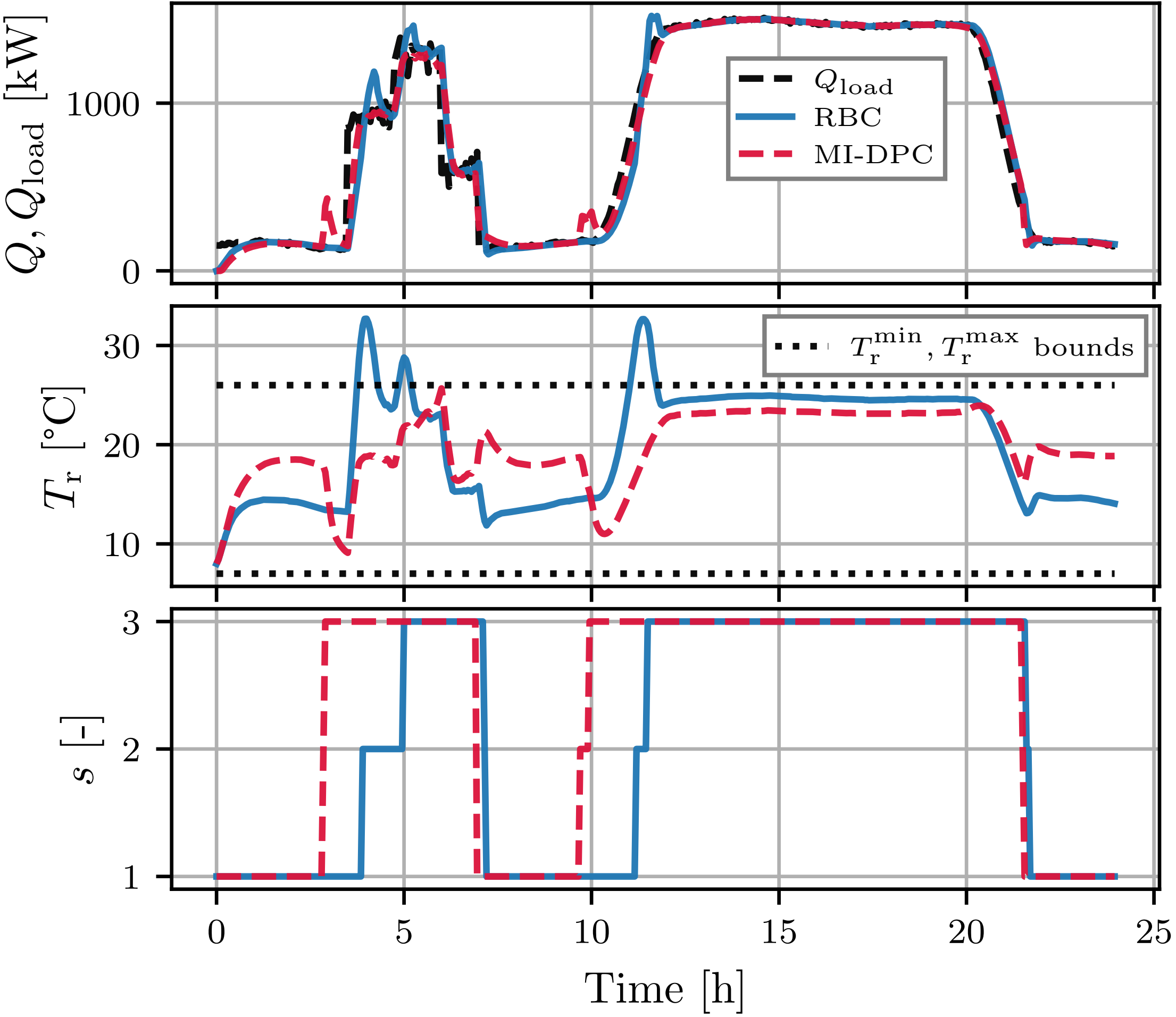
In addition to energy savings, the MI-DPC framework outperformed the RBC in terms of constraint satisfaction. Specifically, when considering cooling ramp-rate constraints, i.e., \(\dot{Q}_{\min}\leq\!\dot{Q}\!\leq\dot{Q}_{\max}\), which have been observed in real chiller plant operations and reported by Shan et al. (2021); the RBC may fail to activate chillers in time when encountering a steep increase in cooling demand. As illustrated in Figure below, the RBC stages chillers solely based on the staging threshold. However, due to the cooling ramp limitation, the return temperature can exceed the process safety bounds. In contrast, the MI-DPC framework anticipates future load changes and stages chillers proactively based on the known future cooling demand. In the experiment, during the \(3\!-\!7\) hours interval, the results demonstrate that MI-DPC effectively adapts to abrupt changes in the cooling load profile, even when such scenarios were not represented in the training dataset.
Simulation results

Figure: Closed-loop simulation results of a chiller plant \( (M\!=\!3) \) with MI-DPC \( (N\!=\!15) \) and RBC policies, highlighting the importance of predictive action for stable operation when cooling ramp-rate constraints are considered.


Computational Scalability
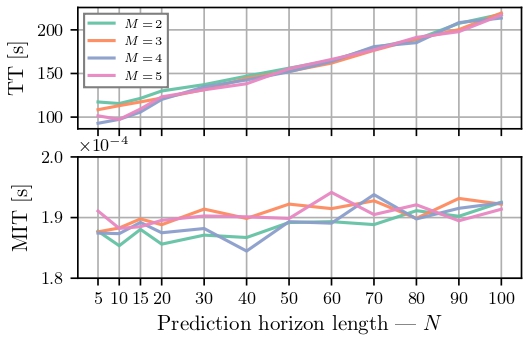
The principal advantage of MI-DPC lies in its computational efficiency during both controller synthesis and inference. Notably, the equivalent MI-MPC formulation was shown to be computationally intractable even for the smallest problem instance with \( M = 2 \) and \( N = 5 \), where, using the Gurobi solver, the mean inference time was around 150 seconds. In contrast, MI-DPC achieves inference times several orders of magnitude faster, enabling mixed-integer nonlinear optimal control problems to be solved on computationally constrained edge devices in real time—a capability not attainable with conventional approaches. The computational scalability of MI-DPC is illustrated in the Figure below.
MI-DPC Computational Scalability Results

Figure: Computational scalability of MI-DPC across different numbers of chillers \( (M) \) and horizon lengths \( (N) \). The top panel illustrates the total training time ( TT ), while the bottom panel reports the mean inference time ( MIT ).


Conclusions and Future Work

This work proposes a mixed-integer nonlinear Differentiable Predictive Control (MI-DPC) framework for real-time optimization of multi-chiller plants, unifying discrete staging and continuous setpoint control within a single differentiable program. In simulations on multi-chiller systems, MI-DPC achieved up to \(13\%\) energy savings relative to an industrial RBC baseline while maintaining process constraints, and delivered orders-of-magnitude faster inference than the equivalent MI-MPC formulation, indicating strong potential for practical and scalable deployment on large-scale HVAC operations.

Building on the findings of this study, several extensions are envisioned. The chiller plant model is to be extended to include cooling towers, allowing for further energy savings potential through optimization of condenser-water loop setpoints (Huang et al., 2017; Wang et al., 2019). The integration of water-side economizers can also be explored, as these have been shown to reduce energy through free-cooling (Faulkner et al., 2025) and introduce additional discrete control variables for economizer activation. Future work will also incorporate probabilistic cooling-load forecasting to more accurately capture real-world uncertainty.

It is further recognized that the problem is solved approximately, without a guaranteed global optimum. Moreover, while integrality and satisfaction of input constraints are enforced through projection-based methods, strict feasibility for state constraints is not guaranteed. These aspects will be addressed in future work.

Acknowledgment

This research was supported by the U.S. Department of Energy Building Technologies Office (BTO), USA within the Office of Energy Efficiency and Renewable Energy (EERE), USA under Contract No. DE-AC05-76RL01830.
PNNL Logo

This work was also supported by the Ralph O’Connor Sustainable Energy Institute (ROSEI) at Johns Hopkins University.
JHU Logo

BibTeX

@article{boldocky2026data,
      title={Data center chiller plant optimization via mixed-integer nonlinear differentiable predictive control},
      author={Boldock{\'y}, J{\'a}n and Faulkner, Cary and Michael, Elad and Gulan, Martin and Tuor, Aaron and Drgo{\v{n}}a, J{\'a}n},
      journal={Control Engineering Practice},
      volume={174},
      pages={107063},
      year={2026},
      publisher={Elsevier},
     doi = {https://doi.org/10.1016/j.conengprac.2026.107063},
    }